A photon in sodium vapour is not travelling. It is waiting.
A resonance photon emitted in a dense vapour is reabsorbed within a fraction of a millimetre by a ground-state atom, held for a natural lifetime τ ≈ 16 ns, and re-emitted in a fresh direction at a fresh frequency. The excitation does not stream out of the cell; it performs a random walk from atom to atom. Holstein's trapping factor g₀ is simply the mean number of hops before escape, and the observable decay slows from \(e^{-t/\tau}\) to \(e^{-t/g_0\tau}\) [Molisch & Oehry p. 3 — read].
Watch it happen. Each spark below is one excitation: it hops with a mean free path drawn from the line profile (frequency redistribution at every hop — long flights in the wings, short stumbles at line centre), and the counter measures g₀ directly as ⟨hops before escape⟩.
FIG 1 Monte Carlo imprisonment in a slab, live. Doppler wings are steep, so g₀ grows ≈ linearly with opacity; Lorentz wings are fat, photons cheat through them, and g₀ grows only as √(k₀L) [pp. 110–111 — read]. At every hop the photon is a 3p atom. Line-centre light has no existence independent of the occupancy — the energy ledger of "trapped radiation" is an atomic ledger.
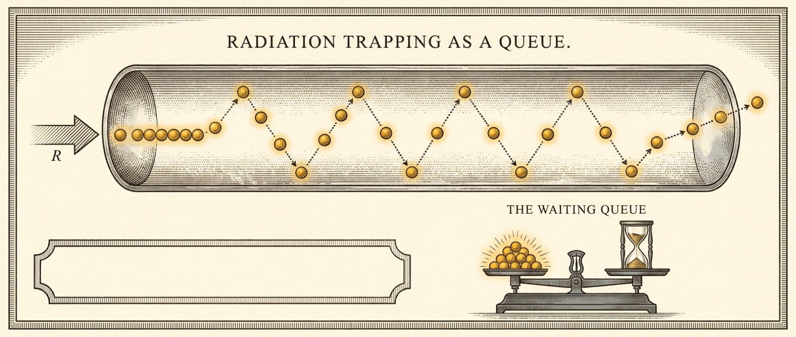
Little's law, for photons.
Now drive the vapour continuously — a discharge, a flame, an electron swarm — at a fixed excitation rate R. In steady state nothing visible decays; what trapping does instead is raise the standing population. The textbook says it in three lines:
"For steady-state problems, the 'visible' physical effect of radiation trapping is not a prolongation of the lifetime… but an increase in the excited-state density… the rate equation becomes Eexc = n₂·A₂₁/g₀. We can easily see that the excited-state density is increased by a factor g₀." MOLISCH & OEHRY, RADIATION TRAPPING IN ATOMIC VAPOURS, P. 6 — READ THE PAGE
This is a queueing identity. Arrivals R, mean residence g₀τ, therefore inventory n* = R·g₀τ. Stored energy Utrap = ħω·n* = ħω·R·g₀τ — linear in g₀ by construction, because g₀ is defined as the residence-time multiplier. Drag the sliders; the dots are individual excited atoms, the ledger is exact.
FIG 2 The queue. Every atom that lights up is an arrival; it stays lit for an exponential residence with mean g₀τ; departures stream off to the right. Halve the wait or double it — the throughput is untouched, only the inventory moves. "More occupied states" and "longer excitation time" are not two effects: at fixed flow, the inventory is the residence time. One ledger entry, two readings.
Two of these are the same notebook page read from opposite ends, and Move IV will show they are the two limits of one curve. But first: in what variable is any of this linear?
τ, T, or n: pick the one the physics is polynomial in.
The trapped state can be parametrized three monotonically-equivalent ways: a longer effective lifetime g₀τ, a hotter excitation temperature Texc, or a larger occupancy n*. Since they move together, you may linearize on any of them. They are not equally honest:
- Occupancy is exact. Utrap = U·n* is an identity — degree one, no expansion, no operating point.
- Lifetime is conditional. n* = R·(g₀τ) is linear only at fixed throughput — Little's law with fine print.
- Temperature is exponential bookkeeping. Texc is defined per transition by nu/nl = (g'u/g'l)e−ΔE/kTexc [pp. 35–36 — read]. Off equilibrium there is no shared Lagrange multiplier: each line pair gets its own Texc, they disagree, and under inversion the number turns negative.
The canonical formalism already voted. The Holstein equation is "a rate equation for the excited-state atoms" — photons are integrated out into a kernel; occupancy is the only dynamical variable [p. 57 — read]. Temperature appears nowhere except inside the Doppler width.
FIG 3 The same physical state under three parametrizations. The curve is stored energy versus your chosen variable; the dashed line is the tangent at the operating point, extended ×2. On occupancy the tangent is the curve — 0% error at any extrapolation. On lifetime it holds while R holds. On temperature the tangent tears away exponentially, and note the two T_exc readouts: the 3s–3p and 3p–3d "temperatures" of the very same vapour disagree — a label per line, not a state function.
Your two equations are one curve with a knee.
Add the one process the pure queue ignores: collisional destruction at rate C (quenching, pooling, wall losses). Per excitation, the photon-destruction probability is ε = C/(C + A/g₀). Steady state for a two-level atom under pump R:
Below the knee, escape is the bottleneck: inventory climbs linearly in g₀ and every pumped quantum still exits as a photon — that is Utrapped = g₀·(UnA₀e−U/kT). Above the knee, collisions pin the population near its Boltzmann anchor and the emerging light falls as Pb/g₀ — the quenching equation of [p. 336 — read]. Both notebook lines are exact asymptotes of this one expression. And the boxed identity is the whole dispute in one line: the elasticity of occupancy with respect to trapping equals the escape branching ratio. Linearizing on g₀ is honest exactly to the extent that β(g₀) ≈ 1 — the slope is the survival.
FIG 4 Log–log: gold = inventory n*(g₀), green = escaping power. Slide C upward and watch the knee g* = A₀/C march left, eating the linear regime. Trapping builds inventory only while radiative escape is the bottleneck; past the knee it merely hands the energy to collisions — which, for a thermally pumped selective emitter, is not loss but thermalization toward Planck at line centre. Pick your side of the knee on purpose.
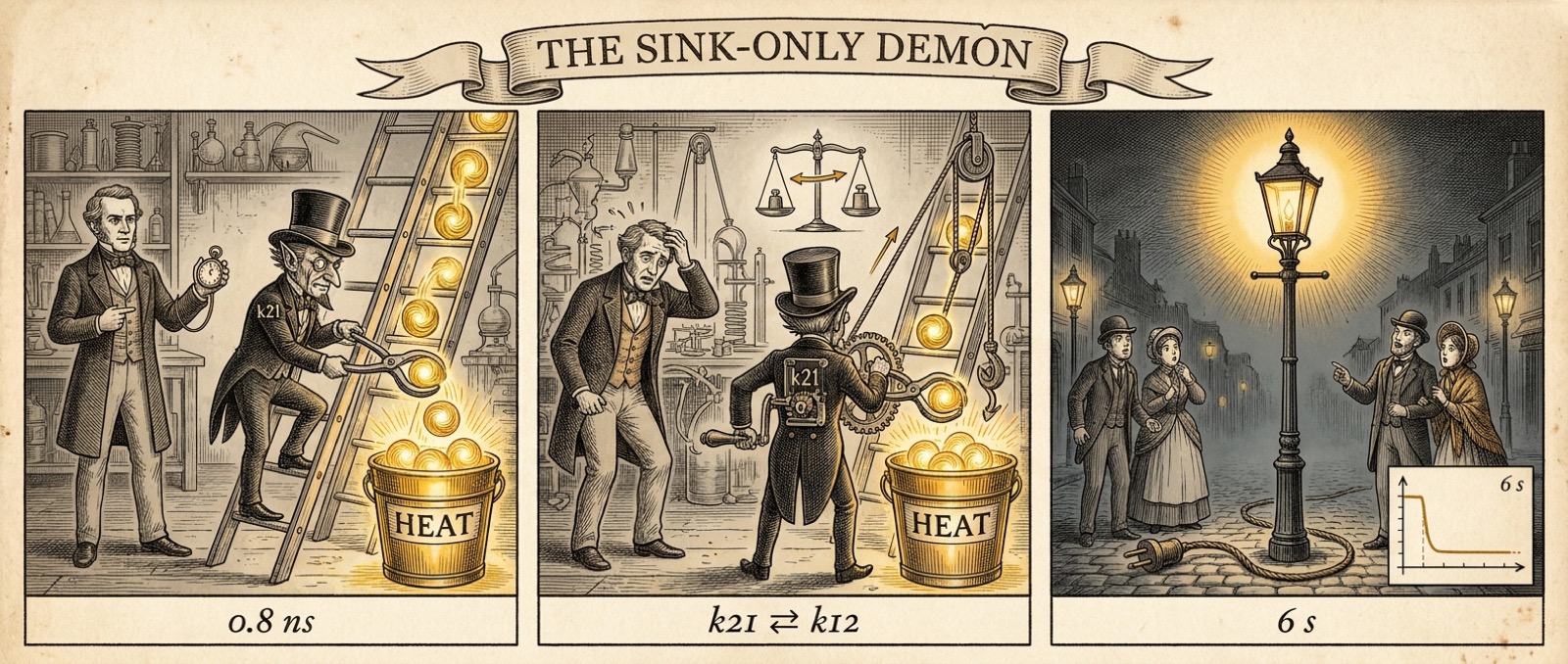
PLATE III The sink-only demon. Panel one is the quenching memo: k₂₁ as a one-way drain, output dead in 0.8 ns. Panel two is detailed balance — the same bath that quenches must re-excite at k₁₂ = k₂₁(g'₂/g'₁)e−ΔE/kT while hot; the demon's crank is not optional (M&O Eqs. 3.6–3.8). Panel three is the published verdict: an HPS lamp, unplugged, still radiating at 589/819 nm seconds later, riding its bath down — de Groot & van Vliet Figs. 3.27–3.28. The ×70 switch-off step in that chart is a direct occupancy measurement: in the Wien regime, optically thick line-center radiance reads g'₁n₂/g'₂n₁ — no temperature appears anywhere in the measurement, which is Move III's point wearing lab clothes.
The boosted occupancy is itself an absorber: 819 nm goes thick.
Here is why occupancy — not lifetime, not temperature — is the load-bearing variable: it is the only one that propagates up the level scheme. The opacity of the 3p→3d line at 819 nm is k₈₁₉ ∝ n(3p) − (g'₃ₚ/g'₃d)·n(3d): degree one in occupancies, including its own bleaching correction. The D-line trapping factor multiplies n(3p); n(3p) buys optical depth at 819 nm; the 819 nm photons begin to trap in turn, and the inventory climbs the ladder [lower state itself excited: p. 60 — read; cascaded trapping: p. 306 — read; measured for Na 3p: p. 329 — read].
And sodium hands you one clean gift: in the HPS arc the D-line is self-broadened, so its own trapping factor is opacity-independent — g₀ = (1/0.211)·(ν₀L/c)1/2, fixed by geometry alone [Eq. 7.14, p. 111 — read]. The escalation lives entirely on the 3p→3d rung, driven linearly by the drive.
Two framings borrowed from the sister plate — attributed, not re-derived here. The mirror heuristic: sodium vapour is opaque at its own line, but opacity is not reflectivity — a useful figure of merit for a sodium mirror is τ×ω, where ω = A/(A+k_Q) is the per-capture survival (the single-scattering albedo). Hot sodium is bright but lossy; cold quench-free sodium reflects — whence their proposed two-chamber geometry: emitting core, vacuum gap, cold ω→1 blanket. The design point: the 819 nm tap saturates its window when τ₈₁₉ through the cool skin reaches 1 — peak extraction at self-reversal onset. The sister plate reports the lab device at τ₈₁₉,skin ≈ 0.004 (≈250× below onset); that number comes from their solver session and awaits independent verification — treat the slider below as exploring claimed, not audited, headroom.
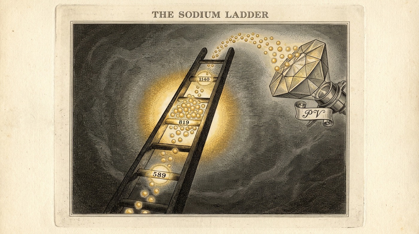
PLATE II The ladder, allegorically. The crowd on the 819 rung is bought with the D-line trapping factor; the leap into the jewel is the PV band.
FIG 5 The sodium ladder, occupancies live. Arrow thickness = photon traffic; halo = trapped inventory; the 819/1140 nm rungs sit exactly at the convertible energies. Turn the bleaching term off to see what a naïve fixed-opacity model overclaims — then notice the correction itself stayed linear in the occupancies. Nothing on this diagram is linear in any temperature.
The afterglow signs the ledger.
Everything above is falsifiable with a pulsed lamp and a photodiode. Kill the drive: the afterglow decays with time constant g₀τ — the residence time, read directly off a scope. The integrated afterglow is the inventory; their ratio is the throughput. One trace yields all three queue quantities. And at high drive the decay departs from a single exponential: pooling drains the inventory as n*², bending the early afterglow downward — the signature that you have left the linear regime, visible before any calibration.
FIG 6 Semilog afterglow, dn/dt = −n/(g₀τ) − βn². The late tail is always the honest single exponential 1/(g₀τ); the early bend is the n² pooling drain — which for an upconverting TPV emitter is not a defect but a pump into the 819 nm ladder of Move V. Cross-check higher modes have died before fitting [p. 56 — read].
The Fong Ansatz: make the occupancy the quantum number.
Tile the vapour into voxels of side λ/4 — the in-phase volume, inside which dipoles cannot dephase geometrically. The ansatz: the voxel occupancy \( m \equiv n_{3p}(\lambda/4)^3 = g_0\, m_B \) is not bookkeeping but the quantum number — a voxel of N atoms holding m excitations is a Dicke state \(|J{=}N/2,\,M{=}m{-}N/2\rangle\), and the trapping factor is how many rungs up the collective ladder the trap loads each coherence volume. This is this page's headline made integer-valued: occupancy = g₀ × Boltzmann, by construction — now per voxel, now countable.
The license for the quantization: the Holstein kernel and the Dicke decay matrix are the same object, \( \Gamma_{ij} \propto \Gamma_0\,\mathrm{sinc}(k r_{ij}) \). Radiation trapping is its incoherent diagonal — photon hops, g₀. Superradiance is its coherent collective eigenvalue — rate \( \Gamma_0\, m(N-m+1) \). One matrix, two faces, one parameter nλ³. And superradiance closes the loop on the queue: collective emission renormalizes \( A_{\rm eff} = A_0(1+m) \), shortening residence, so the steady state solves \( m(1+m) = g_0 m_B \) — the occupancy self-clamps at \( m^* = \tfrac{1}{2}(\sqrt{1+4g_0 m_B}-1) \approx \sqrt{g_0 m_B} \), marginally critical at the quantum threshold.
FIG 7 An actual voxel lattice this time: an 11³ cube of (λ/4)³ coherence volumes, occupancies Poisson-sampled at the clamped m*, depth-sorted and rotating. Gold voxels have crossed m ≥ 1; red cores hold m ≥ 2 (collective). Switch the coherence-volume convention and watch the verdict: the scaling survives every convention, but at the λ̄³ prefactor the same vapour drops below threshold and the gate flips to "dephasing wins." A theory whose verdict depends on an O(1) geometric prefactor is precisely a theory that the pulsed rig must settle.
Are these really voxels? — the kernel honesty
No tiling is the real object. The real object is the collective decay matrix \( \Gamma_{ij} \propto \Gamma_0\,\mathrm{sinc}(k r_{ij}) \), which has no sharp boundary — the voxel is the mnemonic that its coherence range is ~λ/4, and the cube is a diagonal approximation of an eigenvalue problem. Two consequences, both honest. First, the pairwise coherence integral \( \int \mathrm{sinc}^2(kr)\,d^3r \) diverges linearly in an infinite medium: the cutoff is supplied by reabsorption — the same trapping that loads the ladder truncates the coherence volume. Trapping regularizes superradiance; g₀ appears on both sides of the ansatz. Second, extended samples carry the Rehler–Eberly shape factor μ (Fresnel-number physics for pencil geometries): the prefactor in m is convention- and geometry-dependent at the factor-of-four level. What survives all conventions: m ∝ g₀ (the linearization), the existence of a threshold, and the √-clamp. What does not: whether today's operating point sits above or below it.
Four gates, all marginal — counted honestly. (1) Doppler dephasing: N·m*·Γ₀·T₂* ≈ 2.6 at the cube convention. (2) Geometric prefactor: ×1 → ×0.26 across conventions — flips gate 1. (3) Motional churn: a 970 m/s atom crosses the voxel in ≈150 ps while the collective burst takes ≈40 ps — survives, ratio ≈ 0.25. (4) Resonant dipole–dipole: at 10²³ m⁻³ the self-broadening interaction gives T₂ᵈᵈ ≈ 47 ps ≈ t_SR ≈ 38 ps — and since the collective rate and the dephasing both scale with density, this ratio is density-independent: permanently marginal. Note the irony with open eyes: the same interaction that makes g₀ opacity-independent (Eq. 7.14, the ansatz's cleanest feature) is the interaction that dephases the manifold. The ansatz's friend is its enemy, at unit ratio. Status: ansatz; four marginal gates; only the kernel eigenproblem or the pulsed rig can rule. Verification program: three mandates, independent seats, advisor S. Lloyd — in progress.
The pages, deep-linked.
All citations resolve into the full OCR'd monograph hosted on this domain (reader · raw .md · how it was OCR'd).
- Molisch & Oehry, Radiation Trapping in Atomic Vapours, OUP 1999. Trapping factor defined p. 3; steady-state ×g₀ p. 6; detailed balance & Boltzmann anchor pp. 35–36; Holstein eq. as atom rate equation p. 57; eigenmode residence g_jτ p. 56; excited lower states p. 60; self-broadened g₀, Eq. 7.14 p. 111; cascaded trapping p. 306; Na 3p density under trapping p. 329; quenching vs g₀ p. 336; discharge lamps pp. 368–373.
- Holstein, T., "Imprisonment of Resonance Radiation in Gases," Phys. Rev. 72, 1212 (1947).
- Little, J. D. C., "A Proof for the Queuing Formula L = λW," Oper. Res. 9, 383 (1961).
- Companion explorable: Holstein → CRETIN, nine layers from the kernel to the 819 nm extraction calculator.
- Sister plate: "Radiation Trapping, Linearized — the slope is the survival" (sim.lightcellenergy.com) — the β theorem, the τ×ω mirror heuristic, the two-chamber proposal, and the τ₈₁₉=1 design point. The β theorem is independently re-derived on this page; the solver-derived numbers (wall floats, τ₈₁₉,skin ≈ 0.004) are theirs alone and not yet independently audited.
- Sister treatments: plasmagicians.com plate Linearize on Occupancy; book.lightcellenergy.com.